Monday, January 30, 2012

Google Mapplet for showing UTM grid zones

The Universal Transverse Mercator (UTM) coordinate system is a grid based system for specifying locations on the earth's surface. UTM consists of 60 zones, each with its own local Transverse Mercator projection. The Wikipedia site http://en.wikipedia.org/wiki/Universal_Transverse_Mercator_coordinate_system has more information about UTM.

This Google Mapplet was created to display the UTM grid zones and labels on interactive maps. The current version allows the user to change the grid line color for better visualization over different backdrops.

Click this link http://dominoc925-pages.appspot.com/mapplets/utmgrid.html to run the mapplet.

Monday, January 23, 2012

Join a spatial table with a non-graphical table in gvSIG

It is very useful to join a geospatial feature with a related non-graphical database table for analysis. This is a common feature found in commercial GIS applications like GeoMedia. I found a similar function in the open-source software gvSIG although it seems to handle only inner type joins. An example of using the gvSIG Join command is described below.
  1. Start gvSIG OADE. Load and display a geospatial feature e.g. States.shp in a map view.
     
  2. Load a database table e.g. SalesByStates.dbf.


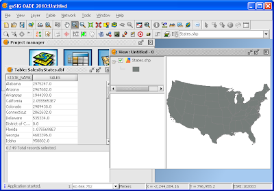
  3. In the Map view legend TOC, click on the geospatial feature name e.g. States.shp. Then press the right button of the mouse on the name.

    A pop up menu appears.
  4. Choose Join.

    The Join tables dialog box appears.

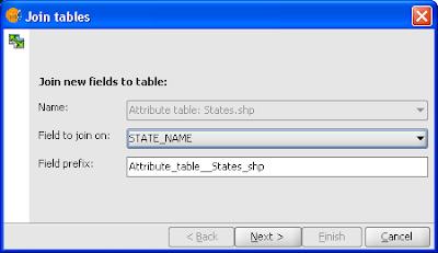
  5. In the Field to join on combo box, choose a common field between the graphical and non-graphical table e.g. STATE_NAME.
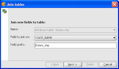
  6. In the Field prefix field, type in the prefix string to indicate the fields from the geospatial feature table e.g. States_shp. Click Next.


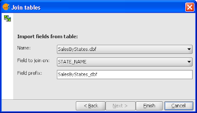
  7. In the Name field, choose the non-graphical table e.g. SalesByStates.dbf.
  8. In the Field to join on, choose the common field between the non-graphical table and the feature table e.g. STATE_NAME.
  9. In the Field prefix field, type in the prefix string to indicate the fields from the non-graphical table e.g. SalesByStates_dbf. Click Finish.


    The tables are joined.
To see the results of the join, you can view the attribute table or query the attributes of selected features. For example, press CTRL+I, then click on any feature in the map view. The Query results dialog box should appear showing the joined table attributes, as shown below.


Monday, January 16, 2012

Connect to non-graphical tabular database data in gvSIG

Being used to commercial GIS software, I was looking around for the option to connect to a non-graphical database table in the gvSIG OADE 2010 application window. I failed to locate the command. Later on, I saw that the command is contained in the Project Manager window - a child form within the main gvSIG application window. Once I found it, it was quite easy to connect to the non-graphical database table as shown in the dbf example below.
  1. Start up gvSIG OADE 2010.
  2. In the Project Manager dialog box, click the Table button.

  3. Click the New button.

    The New table dialog box appears.
  4. Click Add.

    The Open dialog box appears.
  5. Browse and select a dbf file e.g. SalesByState.dbf. Click Open.

    The selected file is added to the list of Tables.
  6. Click OK.

    The attribute table is displayed in gvSIG.

Monday, January 9, 2012

Import a CSV text file into gvSIG

Text files formatted as CSV (comma separated values) are a common data transfer method from system to system. In gvSIG, it is possible to import the CSV files into a binary DBF file through an easy to use graphical interface. Instead of calling the function as Import CSV or something to that order, gvSIG uses the term Normalize Text File.

An example of importing a CSV file into a binary .dbf file is illustrated below.

  1. Start up gvSIG OADE. Open up a View.
  2. Select Table | Normalize text file.

    The Load text file dialog box appears.

  3. Browse and select a CSV file e.g. C:\temp\test.csv. Click Open.

    The Normalization dialog box appears. By default, a new field entry named as NewField is listed.

  4. Click the NewField field. In the Field name field, change the value to a suitable name e.g field1.
  5. In the Separators group box, toggle on Other and type in a comma: ,.
  6. Click the + button.

    A new field NewField2 is added to the list box.
  7. In the Field name field, change the value to a suitable name e.g. field2.
  8. Repeat the previous steps 4 to 7 for each field.


  9. Click Test run.

    A preview of the normalization is displayed in the Sample output field.
  10.  If the preview shows the values have not been separated properly, trace back the previous steps and correct any errors.
  11. If the preview shows the values can be separated properly, click Run.

    The New table dialog box appears.

  12. Browse and type in a new file name e.g. C:\Temp\ImportTest.dbf. Click Save.

    The text file is imported and displayed.


Monday, January 2, 2012

Google Gadget for creating ESRI World Files


Note: A WebApp version of this Google Gadget will be up in a short while to replace this gadget.

The ESRI World file is a text file used to georeference a corresponding image file. A detailed description of the format can be found in this Wikipedia page http://en.wikipedia.org/wiki/World_file.

Recently I had to create ESRI World files for hundreds of aerial photographs, each having different origin, resolution and orientation. As a result of that exercise, I learnt enough about the World File format to create this Google Gadget.

This gadget can help to create the world files given the following input parameters:
  1. X coordinate of the upper left pixel in ground units,
  2. Y coordinate of the upper left pixel in ground units,
  3. Size of the pixel in the X-axis direction in ground units,
  4. Size of the pixel in the Y-axis direction in ground units,
  5. Rotation angle in degrees of the image from North (clockwise is positive) 
Just fill in the required input, click the button and copy and paste the results into a world file, which must be named according to the type of image file. For example, the World file should have the file extension of .tfw for associating with TIFF images.